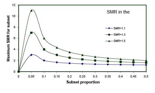
Figure 1: Estimated Maximum Hidden Subset SMR with Population SMR and Subset Proportion Assuming SMR for Remainder of the Population is 1.

Xuguang (Grant) Tao*
Division of Occupational and Environmental Medicine, Department of Medicine, Johns Hopkins School of Medicine, Baltimore, USA*Corresponding author: Xuguang (Grant) Tao, Division of Occupational and Environmental Medicine, Department of Medicine, Johns Hopkins School of Medicine, Baltimore, USA, E-mail: xtao1@jhmi.edu
This paper proposes a simple screening method to detect possible hidden high risks in a subset of a population that has shown low risks in total. Using an example, with the method, the unknown standard mortality ratio (SMR) and its confidence interval for a disease in a subset of a study population could be predicted, given the proportion of the subset and the SMR of that disease in the study population. The confidence intervals calculated for the estimated SMR can be used to judge whether the risk possibly existing in the subset is statistically detectable at the desired significance levels. The method could be a useful tool in suggesting whether a statistically detectable high risk of a disease may be hidden in a subset of a no or low risk population and further study is needed.
Healthy worker effect; Methodology; SMR; Relative risk; Risk screening
Standard Mortality Ratio (SMR) analysis has been very popular in occupational epidemiological cohort studies, in which observed deaths are compared with expected deaths based on the death rates of US general population [1]. One of the advantages of it is that only aggregated information, such as total deaths of the diseases and overall age distribution in the population, is necessary in calculation of SMR. In other words, individual level information is not necessary, although sometimes they data are also available. There is a frequently asked question after SMR analysis has been done for a study population that has shown low overall risks. Is it possible that there is a high-risk subset within the study population simply because the high risk in a subset is diluted when pooling all of the study population together or because of so-called healthy worker effect? Could we miss any risks that appear in a subset that has been exposed to hazardous agents within the study population and what is the maximum risk in that subset we could miss? Is the risk statistically detectable if we do a further study on that subset at a desired significance level? To answer these questions, one usually needs to collect more information on exposures at subset or even individual levels and Poisson regression or Cox proportional hazard models may be used to conduct internal comparisons. However, before the investigators proceed to collect more information and conduct further analysis, is there any way to perform a feasibility screening test to predict the maximum risk in a subset based on limited data and would this risk be statistically detectable? In order to do this, this paper proposes a simple screening method, which might help investigators to decide systematically whether further studies may be needed even though there is no significant risk of diseases in the total study population. An example will be given to show the application of the method used based on a published paper [2].
This screening method should involve two tasks. The first task is to predict the maximum hidden risk and the second task is to estimate the confidence interval of that risk.
If a study population is known to be at low risk of a disease, the risk of the disease for a subset in the study population is then determined by the proportion of the subset in the study population and the risk for the remainder of the study population. The maximum hidden risk for the subset can be estimated by assuming that the risk for the remainder of the population is at a null risk level. If the estimated hidden lower boundary of 95% confidence interval is above one, it suggests that there may be a detectable risk hidden in the subset even though there is no significant risk found in the total study population.
The procedures to identify potentially high risk subsets in a population with no significantly elevated risk compared to an external standard rely on the following assumptions: 1) The remainder of the population outside the selected subset is assumed to be at no excess risk, which means the relative risk equals 1 or standard mortality ratio (SMR) equals 100%. If healthy worker effect is considered a problem, the SMR of a disease for the remainder of the population is assumed to be equal to SMR for all causes of death in the overall study population. It is a widely accepted practice to correct healthy worker effect by assuming the rate for all cause of death as a null value for cause-specific relative risk [3-7]. 2) Confounders such as age are assumed to be homogeneously distributed in the subset and the population for the simplicity of the method introduction. 3) Deaths from the cause of interest are assumed to follow a Poisson distribution, which is a widely accepted assumption [8].
In order to get the estimated SMR for the subset, we need to get the estimated number of cases of a disease and the expected number of cases of a disease. Based on assumptions, the following formulae will stand:
$${{\rm{E}}_{{\rm{subset}}}}{\rm{ = }}\,{\rm{p }}{\rm{.}}\,{{\rm{E}}_{{\rm{total}}}}{\rm{ }}..............\left( 1 \right){\rm{ }}$$
$${{\rm{E}}_{{\rm{nonsubset}}}}{\rm{ = }}\,\left( {1 - p} \right){\rm{ }}{\rm{.}}\,{{\rm{E}}_{{\rm{total}}}}$$
$${{\rm{E}}_{{\rm{total}}}}\,{\rm{ = p}}\,{\rm{. }}{{\rm{E}}_{{\rm{total}}}}\,{\rm{ + }}\left( {1 - p} \right)\,{\rm{. }}{{\rm{E}}_{{\rm{total }}}}$$
$${{\rm{N}}_{{\rm{subset}}}}\,{\rm{ = }}{{\rm{N}}_{{\rm{total}}}}\, - {\rm{SM}}{{\rm{R}}_{{\rm{nonsubset}}}}\,{\rm{. }}{{\rm{E}}_{{\rm{nonsubset}}}}$$
$${{\rm{N}}_{{\rm{subset}}}}\,{\rm{ = }}{{\rm{N}}_{{\rm{total}}}}\,{\rm{ - }}\,{\rm{SM}}{{\rm{R}}_{{\rm{nonsubset}}}}\,{\rm{.}}\left( {1 - p} \right)\,{\rm{.}}\,{\rm{ }}{{\rm{E}}_{{\rm{total}}}}{\rm{ }}...........\left( 2 \right)$$
$${\rm{SM}}{{\rm{R}}_{{\rm{subset}}}}\,{\rm{ = }}{{\rm{N}}_{{\rm{subset}}}}\,{\rm{/ }}{{\rm{E}}_{{\rm{subset}}}}{\rm{ }}.........{\rm{ (3)}}$$
Where,
Esubset: Expected case number of a disease for subset population
p: proportion of the subset of the entire population
Etotal: Expected case of a disease number in the entire population
Enonsubset: Expected case number of a disease for non-subset population
Nsubset: Number of estimated cases of a disease for the subset
Ntotal: Number of observed cases of a disease in the entire population
SMRnonsubset: SMR of a disease for the remainder of the population outside of the subset
SMRsubset: Estimated SMR of a disease for the subset
Formula (1) will be used to calculate the expected case number of a disease for the subset population and formula (2) will be used to calculate the estimated maximum case number of a disease for the subset population. Since p, the proportion of the subset of the entire population, and Etotal, the expected case of a disease number in the entire populationare known, Esubset, the expected case number of a disease for subset in formula one can be easily resolved. In formula (2), Etotal, the expected case of a disease number in the entire population, Ntotal, the number of observed cases of a disease in the entire population, and p, the proportion of the subset of the entire population, are known. The only item which is unknown is SMRnonsubset, SMR of a disease for the remainder of the population outside of the subset. Based on the assumption (1) that the risk of a disease for the remainder of population outside of the subset is assumed to be at null level. SMR for all causes of death in the overall study population is assumed to be that null level, if healthy worker effect is considered a problem. With this assumption, Nsubset, number of estimated cases of a disease for the subset, can be calculated. Finally, SMRsubset, estimated SMR of a disease for the subset, can be calculated using formula (3).
Figure 1 shows the maximum SMR in a subset given the observed SMR of a disease for the total population (SMRtotal), the proportion of the subset (p), and an assumption that the SMR for the remaining population (SMRnonsubset) is equal to 1. For instance, when the SMR for the total population is 1.3 compared to an external comparison, the SMR for a subset which represents 14% of the total can be as high as 3 while the SMR of the remainder of the population is at 1, as shown in Figure 1.

Figure 1: Estimated Maximum Hidden Subset SMR with Population SMR and Subset Proportion Assuming SMR for Remainder of the Population is 1.

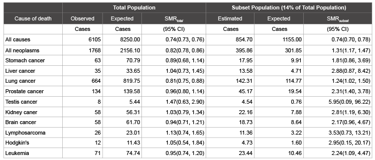
Table 1: Estimated Maximum Subset SMRs and 95% Confidence Intervals of the Example Data*
* Example data for the total population is from [1],
Estimated cases for the subset are calculated using formula (1). Expected cases for the subset are calculated
using formula (2). SMRsubset is calculated using formula (3). 95% Confidence intervals for SMRs of subset are
calculated using formula (4).
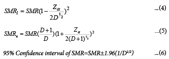
Breslow and Day proposed a method based on the Poisson assumption to calculate the 95% confidence intervals (95% CI) for SMR [9], formula (4) and (5). If the number of cases is larger than 50, 95% CI of SMR can also be calculated using formula (6)

Where,
SMRl : Lower boundary of SMR of a disease in the subset;
SMRu : Upper boundary of SMR of a disease in the subset;
SMR: SMR of a disease in the subset;
Z: Z value of normal distribution;
α : Significance level at 0.05 for 95% CI;
D: Number of expected cases.
The following data is from a published cohort study in an occupational population [2]. The example here includes nine diseases with different numbers of expected death and their SMRs risks. The SMRs were above 1 for five diseases and below 1 for seven diseases including all causes of death. None of the SMRs were significantly higher than 1 compared to the U.S. general population. The question is, “Could we miss any risks within a subset of workers?” For instance, about 14% of the study population was exposed to a certain industrial process, “Other chemical pulping”, chemical puling other than kraft and sulfite pulping. Actually the subset can be defined by any definition, such as a group of workers exposed to a certain product, working area, or group of chemicals. Based on current data could we find out whether there are possible hidden risks in the subset that is 14% of the population? The maximum possibly hidden SMRs in the subset and their confidence intervals are calculated using the methods proposed assuming the null value for risk in the remainder of the population is equal to the all cause of death, 0.74, as shown in Table 1. The results show that a subset, that is 14% of the study population, could possibly have statistically detectable hidden risks for all neoplasms (SMR: 1.31, 95% CI: 1.17, 1.47), lung cancer (SMR: 1.24, 95% CI: 1.02, 1.50), prostate cancer (SMR: 2.31, 95% CI: 1.40, 3.78), kidney cancer (SMR: 2.81, 95% CI: 1.19, 6.30), and leukemia (SMR: 2.24, 95% CI: 1.09, 4.47), if internal comparisons are used in the further analysis, since the all cause of death for the entire study population is assumed as a null risk value in the calculations. The risks in a subset of 14% of the population for stomach cancer, testis cancer, brain cancer, lymphosarcoma, and Hodgkin’s disease, would not be statistically detectable.
The proposed method of analysis is simple and straightforward. The methods will help the investigators to decide whether further studies are needed and would be likely to result in a finding of significant risks in a subset when the overall risk of a disease in the population is not significantly high. Rather than dropping an investigation only on the basis of a total cohort study, using a “shotgun” approach of investigating to screen subsets within the population could be helpful.
In the Dr. Matanoski’s paper [2], The Poisson regression was used to analyze risks for groups of workers exposed to different pulping processes, using internal comparison groups. Among the diseases that were predicted as having possible statistically detectable risks in the subset using screening method in table 1, the relative risk based on the result of the Poisson regression in the previous paper [2] was 1.14 (95% CI: 1.04-1.26) for all neoplasms with “other chemical pulping” process and 1.35 (95% CI: 1.04, 1.75) for lung cancer with “kraft” process, which were very consistent with the predicted levels. Among the disease groups that were predicted as having no statistically detectable risks in the subset, no one showed any significant risks in the Poisson regression analysis except for the brain cancer. Using the method, predicted maximum SMR for brain cancer in the subset was, although not significant, at 2.17 (95% CI: 0.96, 4.67) in table 1. The lower boundary of 95% CI was actually close to 1. The result of the Poisson regression showed a relative risk of 2.33 (95% CI: 1.38, 3.93) with “other chemical pulping”. This discrepancy was probably caused by the violation of one of the assumptions. For instance, the risk for the remainder of the population was probably below the assumed null value.
The null risk value of a disease for the remainder of the population other than the subset in the calculation is assumed to be equal to the risk of all causes of death, if healthy worker effect exists. The healthy worker effect is an observed decrease in mortality in workers when compared with the general population, because of various selection biases and the beneficial effect of work on health. The sources of the selection biases may come from the selection of healthy individuals for employment by an employer or through self selection and from incomplete follow-up due to continuing employment of healthy individuals, and the tendency of those who develop disease to leave employment [1,10,11]. The beneficial effect of work on health could come from physical exertion and the ability to access better medical care, etc. [10]. The healthy worker effect is very common in occupational epidemiologic studies, which tends to bias the relative risk of mortality within industrial working populations downwards by approximately 10-30% below the null value when compared with the general population [10]. Relative risk of a disease in an industrial working population is the combined outcomes of both an upward impact from industrial hazards, if they exist, and a downward impact from healthy worker effect. Because the overall relative risk is far below the general population, the true upward impact from industrial hazards might be compromised by the downward impact from the healthy worker effect. The method proposed in this paper allows users to correct the healthy worker effect by assuming the null value of relative risk of the disease of interest for the remainder of the population is equal to an average, all cause of death, because it is a widely accepted practice to correct for healthy worker effect [3-7].
Download Provisional PDF Here
Article Type: Research Article
Citation: Tao X (2016) A Quick Method for Estimating the Hidden Risks In A Subset of A Low Risk Population. J Epidemiol Public Health Rev 1(2): doi http://dx.doi.org/10.16966/2471-8211.108
Copyright: © 2016 Tao X This is an open-access article distributed under the terms of the Creative Commons Attribution License, which permits unrestricted use, distribution, and reproduction in any medium, provided the original author and source are credited.
Publication history:
All Sci Forschen Journals are Open Access