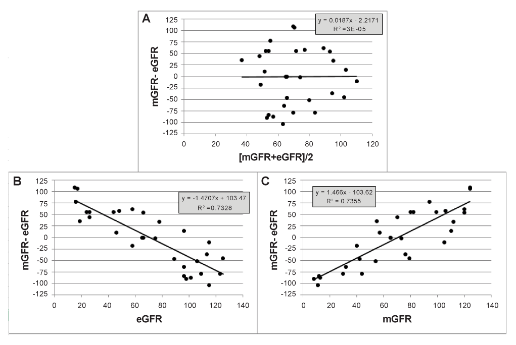
Figure 1: Simulated differences mGFR-eGFR are plotted on averages and on either of both methods, demonstrating the statistical artefact that the difference is related to each of both methods separately.

Hans Potte*
Department of public health and primary care, KULeuven Kulak, Kortrijk, Belgium*Corresponding author: Prof. dr. Hans Pottel, KULeuven Kulak, Department of public health and primary care, Etienne Sabbelaan 53, B-8500 Kortrijk, Belgium, Tel: + 32 56 246022; E-mail: hans.pottel@kuleuven-kulak.be
Background: Bland and Altman have published their method of differences in 1986 in the Lancet to draw their method to the attention of medical professionals. Bland and Altman always have pointed out that their method of differences is designed to detect bias between methods. Their statistical methodology has found its way among clinical chemists, but it has been criticized in 2002 that a high proportion of clinical chemists misinterpreted or misused the methods of differences. It seems that the Nephrology community is falling into the same traps as clinical chemists if they use the method of differences to compare estimating glomerular filtration rate (eGFR) equations with the direct measurement of GFR (mGFR).
Methods: Using simulated data and a real life example, we demonstrate how the method of differences should be used appropriately.
Findings: The main points of criticism are that proportional bias is not analysed correctly and that the calculated 95% limits of agreement should be compared to predefined clinically acceptable limits.
Interpretation: There is no need to introduce ‘alternative’ statistics like absolute mean difference, accuracy within 30%, etc when the BlandAltman methodology is correctly applied. The goal of method comparison is to demonstrate how close the new method is to the (g)old method. The final decision to accept or reject the eGFR-equation is a clinical decision, not a statistical decision. The real problem with currently available eGFR-equations is that none of these equations are close enough to the measured GFR so that the eGFR-equation can replace the measured GFR.
Bland-Altman methodology; Proportional bias; Estimating glomerular filtration rate; 95% limits of agreement
In 1986, Bland and Altman published “Statistical methods for assessing agreement between two methods of clinical measurement” in the Lancet [1], to draw their method, earlier published in the Statistician [2], to the attention of medical professionals. It has been cited more than 30000 times since then. In that article, Bland and Altman described their method of differences for analysing method comparison studies. The method consists of plotting the differences between the values resulting from the two methods of measurement (Y) against the average of the values (X). The statistical analysis that should be performed on this plot evolved over some 16 years [3,4]. Bland and Altman always have pointed out that their method of differences is designed to detect bias between methods. The method has found its way among clinical chemists, but it has been criticized in 2002 that a high proportion of clinical chemists misinterpreted or misused the methods of differences [5].
The main points of criticism were:
a) the x-axis only contained one of both methods, not the average of both methods;
b) the 95% limits of agreement (LOA) were not compared to a predefined clinically acceptable difference between the two methods and
c) the 95% LOAs were not calculated with the appropriate statistical methodology, especially when proportional bias is present.
Although the first point of criticism was addressed in 1995, when Bland and Altman published yet another article in the Lancet [6], entitled “Comparing methods of measurement: why plotting difference against standard methods is misleading”, it seems that the Nephrology community is falling into the same traps as clinical chemists if they use the method of differences to compare estimating glomerular filtration rate (eGFR) equations with the direct measurement of GFR (mGFR). In their 1995 article, Bland and Altman argued that plotting the differences against either of both methods, even in case one of the methods was the standard method, are not the appropriate way to analyse method comparison data. They actually wrote: “It would be a mistake to plot the difference against either value separately because the difference will be related to each, a well-known statistical artefact.”
Bias and other method performance measures have been calculated numerously in the last ten years when comparing eGFR-equations with the direct measurement of GFR (mGFR), but also when comparing eGFR-equations with each other. In most of the published articles on that subject, Bland-Altman plots are used, but mainly only constant (or fixed) bias is reported. The analysis of proportional bias is circumvented by defining eGFR or mGFR-strata and calculating the method performance characteristics in these strata. However, defining strata means that the X-variable becomes involved in the analysis, and then the above referenced statistical artefact comes into play. We here demonstrate how method comparison should be performed, using eGFR and mGFR data, and draw attention to the possible pitfalls of this analysis and more specifically to the above mentioned three points of criticism.
In a first section, we present simulated data and statistical analyses on these data to demonstrate the statistical artefact referenced in the introduction.
In a second section, we use a real life example obtained from the article of Gagneux-Brunon et al. [7] on n = 203 HIV patients for whom the gold standard inulin method has been used to obtain direct measurements for the glomerular filtration rate (mGFR), but also estimated GFR was obtained from serum creatinine, gender and age for different equations (MDRD, CKD-EPI). We analysed the data according to the method of differences described by Bland and Altman [1-4] and John Ludbrook [8- 10].
We here describe the procedure that should be used:
a) Calculate the mean of the ratio eGFR/mGFR and the 95% Confidence Interval (CI) of that mean. When the value ‘1’ is included in the 95% CI, there is no evidence for proportional bias; if not, there is evidence for the presence of proportional bias.
b) Construct a XY-scatterplot of differences (mGFR-eGFR) on averages (mGFR+eGFR)/2. If the slope of the regression is shown to statistically differ from zero, there is proportional bias; if not, there is no proportional bias.
bias ± (t0.05, n-1) × SD.
The value t0.05, n-1 tends to 1.96 when n → ∞.
The method to calculate V-shaped 95% LOAs in case of proportional bias or heteroscedasticity is described by Ludbrook [10] who by chance came across a website in which Bland and Altman [11] described how to calculate this. The steps are as follows:
difference = A + B × average
absolute residual = a + b × average
SD = 1.2533 a + (1.2533 b) × average
or
A + B × average ± 1.96 × (1.2533 a + (1.2533 b) × average)
The statistical artefact mentioned by Bland and Altman can easily been illustrated by randomly generating eGFR and mGFR values. We therefore used the RANDBETWEEN (1,125) worksheet function in MS Excel to generate 30 random numbers between 1 and 125 for eGFR, and independently for mGFR. These random values are assigned to 30 hypothetical patients in a paired way, so that each patient has an eGFRvalue and a mGFR-value which are random and completely independent from each other. For each hypothetical patient, the difference mGFR-eGFR is then plotted against the average [mGFR+eGFR]/2 (Figure 1a), but also against eGFR and mGFR separately. As eGFR and mGFR were randomly generated, independent of each other, no relation exists between eGFR and mGFR, which is also apparent when plotting differences on averages. However, when plotting the difference mGFR-eGFR against eGFR (Figure 1b), the obtained pattern showed a striking linear relationship (R2 = 0.7328, p < 0.0001) with a negative slope. When plotting the difference mGFR-eGFR against mGFR, we observe an increasing linear trend line (positive slope, R2 = 0.7355, p < 0.0001) (Figure 1c). This is entirely an artefact of data analysis. Graphing a difference between methods against either method separately is quite misleading. Attributing a significant correlation on such a graph to method association is termed regression fallacy. Such a plot should not be analysed by linear regression because these data violate one of the assumptions of linear regression, that the X and Y variables were determined independently [12].
In fact, there is nothing wrong with plotting differences against one of the variables separately, unless we start analysing the data and we involve the X-variable in the analysis. In case we are performing regression analysis, we are violating one of the basic assumptions of linear regression, that the X and Y variables were determined independently. But also performing subgroup analysis, by stratifying on mGFR or eGFR, is misleading, because the choice of the subgroup is not independent from the variable under study. Moreover, subgroup analysis is performed as a replacement for analysing proportional bias. In case there is absence of proportional bias, subgroup analysis should present approximately equal fixed biases in each subgroup. In our example, where the values of both methods are obtained by a random number generator, the bias equals zero (Figure 1a). However, subgroup analysis, based on eGFR will give positive bias when eGFR< 60, and negative bias when eGFR> 90, while the opposite is true when mGFR is used to define subgroups (negative bias when mGFR< 60 and positive bias when mGFR>90).
In the opposite situation when proportional bias is present in the differences on average plot, then this bias may be hidden when differences or plotted against one of both methods, due to the same statistical artefact.
We start from an example using a dataset of n = 203 HIV patients [7] for whom GFR was measured directly using the inulin methodology (mGFR) and estimated from different so-called estimating equations (eGFR). We compare the eGFR-MDRD equation with the direct GFR measurement (mGFR), using the Bland-Altman methodology described in the methods section.
Step 1. Calculating the mean of the ratio eGFR/mGFR, we find 1.042 with 95% CI [0.996 – 1.088] from which we conclude that there is no proportional bias, as ‘1’ is included in the 95% CI. Plotting the ratio eGFR/mGFR against the average (Figure 2a) also reveals the presence of 2 outliers in the low GFR region. When omitting these outlying observations, the mean ratio becomes 1.027 with 95% CI [0.986 – 1.069] which does not change our conclusion that there is no proportional bias. Plotting the differences against the average and performing regression analysis gives R2 = 0.0245 with p = 0.026, indicating a small but statistically significant increasing trend in the data (Figure 2b). Omitting the two outliers from this analysis reduces the R2 from 0.0245 to 0.0157 and returns the borderline significance into non-significance (p = 0.075). As both methods to evaluate the presence of proportional bias are not completely equivalent, and because the observed trend is extremely small, we conclude that the proportional bias is relatively small and may therefore be ignored. The least squares methodology is heavily influenced by the leverage effect due to squaring of the deviations. Calculating the mean of eGFR/mGFR balances deviations from ‘1’ under and above this value, just like calculating the mean of mGFR-eGFR balances positive and negative deviations. In this sense, the calculation is very analogous and is the preferred way to indicate the presence or absence of proportional bias. It is really like comparing the data with the identity line when plotting eGFR against mGFR (but without performing regression analysis): the identity line goes through zero (and this is equivalent to zero constant bias) and has a slope of ‘1’ (equivalent to a ratio eGFR/mGFR equal to ‘1’, an indication of the absence of proportional bias).
When plotting the same differences mGFR-eGFR against either of both methods (eGFR or mGFR) we observe the effect explained by Bland and Altman and described in the first part of the results section. When mGFR-eGFR is plotted against eGFR, there is an observed negative trend (Figure 2c), but when plotted against mGFR, there is an observed positive trend (Figure 2d). In both cases, the trends are much more pronounced (and statistically significant) than when plotting the differences against the average.
Analysing the proportional bias is required to calculate 95% LOAs, but it involves regressing mGFR-eGFR against the X-variable. In that case, the plots of differences against one measurement can be seriously misleading. In the example shown, we may conclude that there is a significant negative (or positive) proportional bias, while in fact, there is none.
Step 2. The calculation of the 95% LOAs depends on the presence or absence of proportional bias. Ultimately, the 95% LOAs should be compared to clinically acceptable limits. The final decision to accept the new method, to replace the (g)old method, is not a statistical one but a medical or clinical one. The correct calculation of 95% LOAs is therefore of great importance. This calculation involves the X-variable in the analysis in case of the presence of proportional bias. The way to calculate 95% LOAs in the presence or absence of proportional bias has been described in the methods section.
If we accept that there is no proportional bias (as is indicated by the equality of eGFR/mGFR with ‘1’), then 95% LOAs for the difference on average could be calculated using bias ± 1.96 × SD = [-48; 50 ml/min/1.73 m2 ] which are fixed over the complete range of average values.
Steps 3-4. If we assume now, for the sake of this example, that there is proportional bias, as suggested by the small but statistically significant R2 = 0.0245, then Ludbrook [10] describes a methodology to calculate V-shaped limits for the regression of differences on averages (see methods section) [Figure 3]. The results for our example are shown in Figure 3. Around 50 ml/min/1.73 m2 the MDRD method shows an imprecision resulting in a possible range of differences between mGFR and eGFR varying between -35 to 18 ml/min/1.73 m2 . This prediction range increases to -48 to +50 ml/min/1.73 m2 at the 100 ml/min/1.73 m2 level.
Yet another approach would be to plot the relative differences against the averages. The reason for doing this is that relative differences are probably easier to interpret clinically, in terms of clinically acceptable limits as a % relative difference: e.g. a clinically acceptable limit could be defined as a maximum of 15% deviation. These limits could then be plotted on the Bland-Altman plot, together with the 95% LOAs and make a direct comparison possible.
In figure 4 the effect of the two outliers, previously determined, is clearly visible. Removing these outliers has a serious effect on the form of the V-shape. Assuming absence of proportional bias in this relative difference plot would result in fixed 95% LOAs of [-50% to +52%], not much different from the slightly increasing LOAs in figure 4 (right side).
Step 5. Visual inspection of Figure 4 shows that the clinically acceptable limit of ±15% are much smaller than the actually obtained 95% LOAs, meaning that the MDRD method is not capable of accurately predicting the mGFR. The conclusion of this method comparison study should therefore be that the MDRD method could not replace the (g)old mGFR method.
Scientists are clever and creative. This can also be seen when going through the most recent literature dealing with the evaluation of new equations for estimating GFR. To circumvent the problem of the presence of proportional bias and the more complex calculation of V-shaped LOAs, it has been recommended [13] to calculate bias and other performance measures (e.g. accuracy (P20, P30)) in so-called GFR-strata. These GFRstrata are typically (but not exclusively) defined as
Accuracy defined as P30 is the % within 30% of the measured GFR value, or in other words, the percentage of patients with |mGFR-eGFR|/ mGFR<0.30.
Defining GFR-strata also involves the X-variable in the analysis, as subgroup analysis may be seen as a replacement for analysing proportional bias. When proportional bias is absent, there is no need for calculating (constant) bias in subgroups, as these are all expected to be very equivalent to the overall constant bias. This is demonstrated in Figure 5a and in Table 1 for subgroups defined based on (mGFR+eGFR)/2.
Figures 5b and 5c demonstrate the effect on bias calculation in subgroups based on eGFR or mGFR to define GFR-strata. When choosing eGFR to define GFR-strata, eGFR becomes involved in the data-analysis. As the known statistical artefact predicts a negative proportional bias (negative trend for the difference against eGFR), the bias will be higher in the low GFR-stratum than in the high GFR-stratum, while this will be reversed when mGFR was used to define GFR-strata. The calculated biases are shown as horizontal lines in the figures for each stratum and are given in Table 1.

Figure 1: Simulated differences mGFR-eGFR are plotted on averages and on either of both methods, demonstrating the statistical artefact that the difference is related to each of both methods separately.
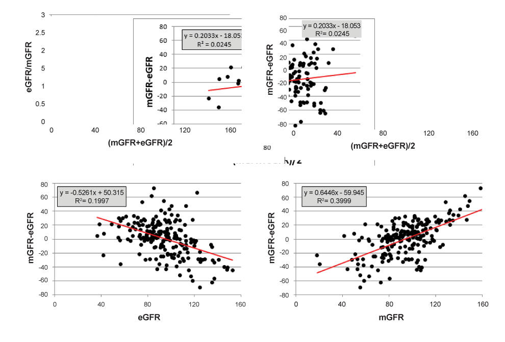
Figure 2: a. The ratio eGFR/mGFR against the average of both methods. Proportional bias is indicated as the deviation from ‘1’. b-d. Difference mGFR-eGFR against average and against both of the methods separately.
The calculated biases in subgroups defined by either eGFR or mGFR are misleading and completely a consequence of the described statistical artefact.
Subgroup analysis for P30
When plotting [mGFR-eGFR]/mGFR against the average of both methods (Figure 6a), or against eGFR (Figure 6b) or mGFR (Figure 6c), the limits corresponding to ± 30% define the area in which the patients within 30% of the mGFR are falling. This analysis is close to the analysis of relative differences, but not exactly the same, as relative differences in Figure 4 were calculated as the differences divided by the average of both methods.
When GFR-strata are defined based on the average, eGFR or mGFR, the results are very different. Strata defined by eGFR or mGFR are very misleading as they suggest the presence of proportional bias, as can be observed by inspection of Figures 6b and 6c.The P30 values are presented in Table 2.
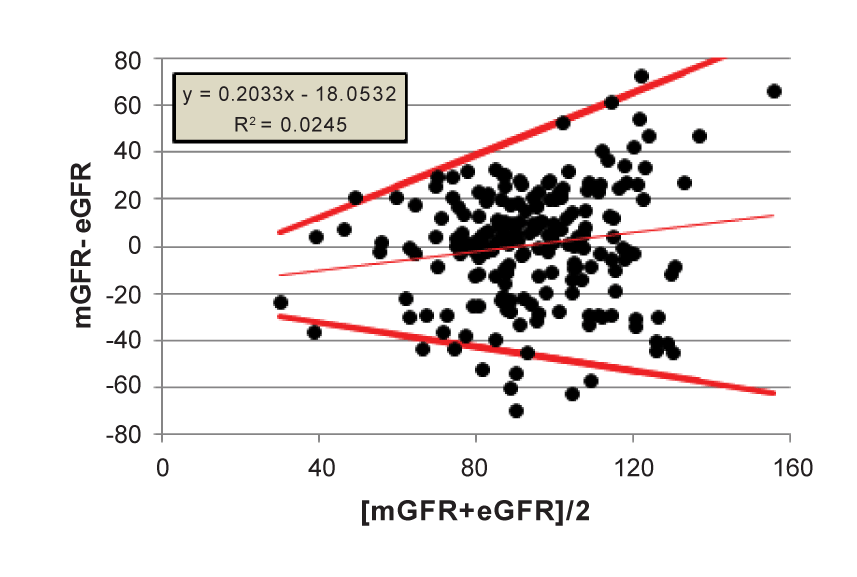
Figure 3: V-shape limits for the regression of differences on averages (Ludbrook7 )
Stratum |
[mGFR+eGFR]/2 |
Egfr |
mGFR |
<60 ml/min/1.73 m2 |
-0.7 |
+8.2 |
-26.7 |
60 ≤ GFR ≤ 90 ml/min/1.73 m2 |
-2.9 |
+9.9 |
-7.1 |
>90 ml/min/1.73 m2 |
+3.9 |
-5.7 |
+9.9 |
Table 1: Bias according to different GFR strata
Stratum |
[mGFR+eGFR]/2 |
eGFR |
mGFR |
<60 ml/min/1.73 m2 |
63 |
50 |
22 |
60 ≤ GFR ≤ 90 ml/min/1.73 m2 |
71 |
83 |
75 |
>90 ml/min/1.73 m2 |
78 |
72 |
83 |
Table 2: P30 (%) according to different GFR strata
An alternative to using P30 would be to make use of the relative differences as explained in Figure 4 and compare the obtained 95% LOAs against clinically acceptable limits.
The goal of method comparison studies is to determine whether the new method (eGFR) may replace the (g)old method (mGFR). In other words, to evaluate whether the two methods of measurement agree sufficiently closely. Statistical methodology may help to present and summarize the available data but ultimately the decision whether to accept or reject the new method is a clinical one. Interpretation of the Bland-Altman plots should be done by comparison of the observed limits of agreement to predefined clinically acceptable limits. Bias and imprecision may be unacceptably high, which may affect the clinical decision for an individual patient, and therefore, the new method may be rejected.
Most importantly, the statistical methodology to compare two methods should be used appropriately. It seems that researchers comparing eGFRequations to mGFR fall into the same traps as clinical chemists a decade ago, if they use the method of differences [5,10]. Bland and Altman’s original goal was to detect bias. Bias, however, can take one (or both) of two forms: fixed or constant bias and proportional bias. Fixed bias means that one method is consistently higher (or lower) than the other method, across the whole range of measurement. This is indicated by a departure of the mean difference from zero. Unfortunately, the mean of differences can also be zero due to the presence of proportional bias, when positive and negative differences are cancelling out each other. Proportional bias is present when the difference in values resulting from the two methods are decreasing or increasing in proportion to the average values. Heteroscedasticity (the scatter of differences is increasing with increasing average) is yet another problem that should be tackled during method comparison studies in an appropriate way. The statistical analysis should result in the correct calculation of 95% Limits of Agreement, which should then be compared to clinically acceptable limits. This is the ultimate goal of method comparison. Once it is decided that the new method may replace the old method, there is no further need for method comparison studies. This is contrary to what is happening in eGFR method comparison studies, where multiple method comparison studies are performed with continuous new cohorts of patients. In 2012 there appeared a systematic review [13] on method comparison studies to evaluate the performance of (mainly) the MDRD Study equation and the CKD-EPI equation to estimate GFR. This review article identified 23 method comparison studies based on serum creatinine assays traceable to SRM (serum reference material). However, their search yielded 3250 abstracts on this subject. The conclusion of this review article was that neither the CKD-EPI nor the MDRD Study equation is optimal for all populations and GFR ranges. This is a euphemism for saying that the CKD-EPI and MDRD Study equation do not fulfil the clinically acceptable limits, because bias and (mainly) imprecision are simply unacceptable. This same review made an (appreciated) attempt to suggest criteria for developing and validating GFR estimating equations. The authors proposed that measures of equation performance should include bias, precision and accuracy and they encourage researchers to report P30 and P20. A relative reduction in bias of 50% or RMSE (root mean square error) of 20% in relevant age and GFR-strata was presented as the goal to achieve. The same authors presented median difference and 1-P30 in eGFR-strata [14]. However, this is not the way method comparison statistics should be applied. Rule [15] criticized the fact that in some studies mGFR-strata were used. He referred to Motulsky [11] to argue why eGFR-strata should be used instead of mGFR-strata. He argued that mGFR-strata could not be used because eGFR-mGFR will have a negative trend with higher levels of mGFR, a fact that we here identified as the regression fallacy. It should be noted that exactly the same arguments can be used to show that eGFRstrata are not appropriate. Both choices are misleading as explained in the results section of this study. Arguing that, from a clinical perspective, it is not helpful to assess equation performance across levels of mGFR because if you know mGFR you would not need to estimate it, and use this argument to state that equation performance should be assessed across levels of eGFR, is difficult to understand. The goal of a method comparison study is either to accept or to reject the new method for replacing the old method. When the new method is acceptable, there is no further need for measuring mGFR, because the estimated GFR is reliable and close enough to the mGFR. This is exactly what happened when enzymatic serum creatinine replaced Jaffe type assays. The enzymatic assay results were compared to the gold standard (IDMS) and it was concluded that the new method (enzymatic assay) was close enough to the gold method. The fact that we may not conclude this for eGFR methods is the real problem.
In the same article, the author explains how “absolute bias” (the mean of absolute value of differences) should be interpreted. Introducing statistical concepts like the absolute bias have only one purpose: to circumvent the problem of proportional bias, as absolute bias is used because positive and negative differences may cancel out each other. There is no need to introduce ‘new’ definitions of bias when proportional bias is analysed appropriately
The group of Levey [13,14,16-22] have dictated that it is preferable to evaluate equation performance based on eGFR rather than on mGFR to minimize the effect of regression to the mean, and others claim that mGFR should be used because mGFR is the (g)old standard method. Both are misleading. Differences between methods should be plotted on averages, not on either of both methods. Bias and accuracy (P10,P30) in eGFR and mGFR-subgroups should not be calculated, as they are misleading. The subgroups should be defined as (eGFR+mGFR)/2-strata. In this sense, we should preferably refer to bias and accuracy in ‘GFR-subgroups’ or at specific ‘GFR-levels’. These levels should be defined based on the average of both methods.
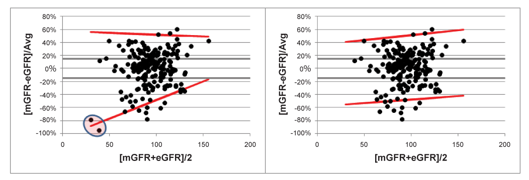
Figure 4:V-shaped 95% LOAs with and without 2 outliers. Clinically acceptable limits of 15% are drawn to make a direct comparison possible with the 95% LOAs.
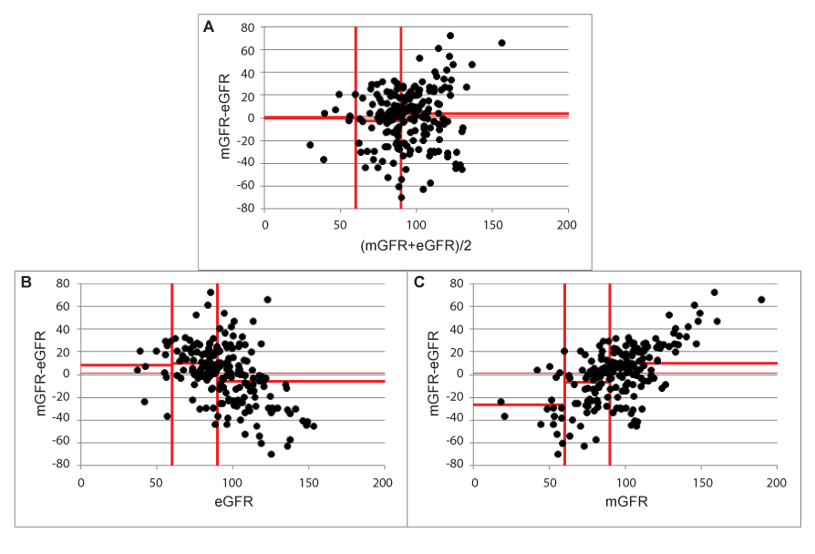
Figure 5:Effect on bias in subgroups defined by (mGFR+eGFR)/2, eGFR and mGFR.
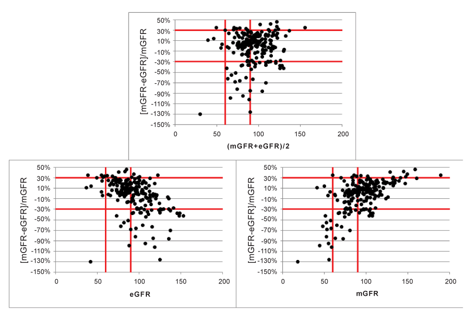
Figure 6:Effect on P30 in subgroups defined by (mGFR+eGFR)/2, eGFR and mGFR.
The problem with method comparison studies to evaluate the performance of eGFR equations is that we cannot decide to ‘reject’ the eGFR-equation because the alternative is the cumbersome and complex direct measurement of GFR. Therefore, we continue using eGFR-equations that are far from optimal and that we continuously evaluate. This has led to a mass production of articles on that subject and it will probably lead to a mass production of articles on that subject in the coming years.
Download Provisional PDF Here
Article Type: Research Article
Citation: Pottel H (2015) Critical Review of Method Comparison Studies for the Evaluation of Estimating Glomerular Filtration Rate Equations Int J Nephrol Kidney Failure 1 (1): doi http://dx.doi.org/10.16966/ ijnkf.102
Copyright:© 2015 Pottel H. This is an open-access article distributed under the terms of the Creative Commons Attribution License, which permits unrestricted use, distribution, and reproduction in any medium, provided the original author and source are credited.
Publication history:
All Sci Forschen Journals are Open Access